Three ways to find out if your water is haunted…

Total organic carbon (TOC) is a bulk measurement that indicates the amount of organic matter in a water. However, properties of organic matter can vary widely. You may have heard terms like “humic” or “fulvic” fractions to describe different types of TOC. There are several analytical methods that can help uncover different TOC properties, such as fluorescence or size fractionation. But for most water treatment plants, we’re concerned about two main questions: TOC removal and disinfection byproduct (DBP) formation. Using historical data directly can be challenging because there are many water quality and operational parameters that impact how well TOC is removed and how much DBPs will form. Luckily, we have empirical models that can help understand plant performance and correct for these factors.

This description assumes you already have a basic knowledge of tidywater. If you don’t know how to create a water or how to connect functions togethers, start with the “getting started” vignette.

We’ll start by looking at these functions for one condition. We’ll begin by defining a water that has all the parameters we need for modeling.

start_water <- define_water(ph = 7.4, temp = 12, alk = 80, tds = 100,
                          toc = 3, doc = 2.8, uv254 = .1, br = 50)

summarize_wq(start_water, params = c("general"))

General water quality parameters Result Units pH 7.40 - Temp 12.00 deg C Alkalinity 80.00 mg/L as CaCO3 Total_Hardness NA mg/L as CaCO3 TDS 100.00 mg/L Conductivity 156.25 uS/cm TOC 3.00 mg/L

The two functions we’ll be using today are:

• chemdose_toc, which predicts the TOC removal from coagulation using the Edwards (1997) model.

• chemdose_dbp, which predicts the DBP formation from disinfection using the Amy model.

We also use chemdose_ph to account for pH changes from chemical addition. Often, we don’t need this function when we’re dealing with historical data because we have real measured pH at different points in the treatment process.

coag_water <- start_water %>%
  chemdose_ph(alum = 30) %>%
  chemdose_toc(alum = 30)

fin_water <- coag_water %>%
  chemdose_ph(naocl = 4) %>%
  chemdose_dbp(cl2 = 2, time = 2, treatment = "coag")

Warning in chemdose_dbp(., cl2 = 2, time = 2, treatment = "coag"): Temperature
is outside the model bounds of temp=20 Celsius for coagulated water.

Warning in chemdose_dbp(., cl2 = 2, time = 2, treatment = "coag"): pH is
outside the model bounds of pH = 7.5 for coagulated water

print(paste("Coag DOC =", round(coag_water@doc, 1), "mg/L"))

[1] "Coag DOC = 2.1 mg/L"

print(paste("TTHM =", round(fin_water@tthm), "ug/L"))

[1] "TTHM = 18 ug/L"

So we can get some model outputs, but how does this tell us anything about our water? For that, we need to look at our historical data. We created some example data, but for a real analysis, this is when you would need to do data read-in and cleanup.

This first question we want to answer (to know if our water is “haunted”) is: Is my TOC hard to remove? By answering this question, we can understand the applicability of these empirical models and whether additional treatment (such as pre-ozone) would help. To answer this question, we want to apply chemdose_toc to our historical data using the _chain family of functions. First, we’ll have to set up the columns, including a new UV column. Since we don’t have historical UV data, we can assume a SUVA and calculate UV.

Note that we don’t use chemdose_ph in this case because we have the coagulation pH in our historical data. We’re also treating TOC and DOC as interchangable because they are usually close and DOC wasn’t measured.

colnames(hist_data)

[1] "raw_toc"   "fin_toc"   "coag_ph"   "fin_ph"    "cl2_dose"  "alum_dose"
[7] "tthm"     

coag_model <- hist_data %>%
  # Creating new columns to feed into define_water_chain
  mutate(doc = raw_toc,
         ph = coag_ph,
         alum = alum_dose) %>%
  mutate(suva_raw = 2,
         uv254 = suva_raw / 100 * doc) %>%
  define_water_chain("precoag") %>%
  chemdose_toc_chain("precoag", "coag") %>%
  # Pull out parameters of interest
  pluck_water("coag", "doc")

Warning: There were 36 warnings in `mutate()`.
The first warning was:
ℹ In argument: `precoag = furrr::future_pmap(., define_water)`.
Caused by warning in `...furrr_fn()`:
! Missing value for alkalinity. Carbonate balance will not be calculated.
ℹ Run `dplyr::last_dplyr_warnings()` to see the 35 remaining warnings.

# Plot actual vs modeled coagulated DOC

ggplot(coag_model, aes(x = fin_toc, y = coag_doc)) +
  geom_point() +
  geom_abline() +
  coord_cartesian(xlim = c(0, NA), ylim = c(0, NA)) +
  theme_bw() +
  labs(x = "Actual TOC", y = "Modeled TOC")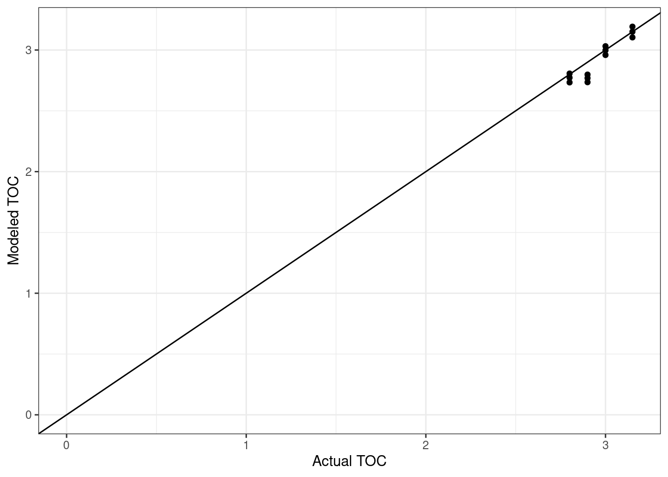

In a plot like this, anything above the 1:1 line means that the model is predicting “worse” removal than we are actually seeing and below the 1:1 line means that the model is predicting “better” removal. So if most of your data is below the line, your TOC is more recalcitrant to removal than the waters used to create the model - more “challenging” than a typical source water. If you are close to the line, you can use the model to get a pretty good prediction of coagulation performance.

The next question we want to ask is: Are there conditions that make my TOC easier or harder to remove?